
Research · Methodology + tooling · 2026
Batch2go: isolating batching effects by placement

Primary artifact · GitHub
matthewhoung/batch2go
The proxy, the three controlled conditions, the run harness and the matplotlib analysis pipeline. C1, C2 and C3 are byte-frozen at a release tag; every result cell carries a completion marker so a run can be resumed idempotently, and each session writes a machine-readable manifest.
Serving systems batch requests at more than one point in the stack: an upstream component may aggregate before transmission, and the inference server may batch again at execution. Conventional end-to-end evaluation sees only the sum, which conflates transport-layer aggregation with compute-layer parallelism. This work treats batching placement as an isolable architectural variable, with three controlled conditions — a no-batching baseline (C1), a compute-layer control (C2) and a transport-layer treatment (C3).
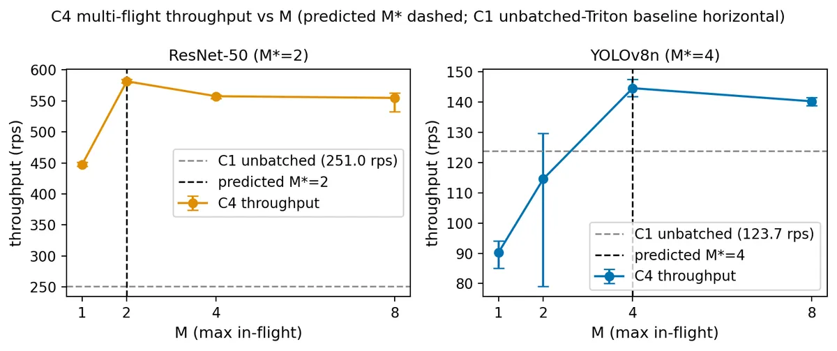
The conditions are instantiated by Batch2go, a single-flight Go proxy that decomposes batch cycle time into a compute service time Sk and a transport overhead Dk. Single-flight execution is what makes the decomposition possible at all: it defines a regime in which Sk and Dk are separately observable rather than entangled in one aggregate measurement. Those two quantities then predict the upstream concurrency for a composed multi-flight deployment as M* = ⌈Dk/Sk⌉ + 1 — a number derived from the decomposition before any multi-flight configuration had been run.
研究摘要
這個研究把「batching 發生在哪一層」當成一個可以單獨控制的架構變數。傳統的 end-to-end 量測只看得到總和,分不出傳輸層的聚合跟計算層的平行化各自貢獻了多少。
Batch2go 是一個 single-flight 的 Go proxy,把一個批次週期拆成計算時間 Sk 跟傳輸開銷 Dk。拆開之後就能事先算出上游應該開多少並行度,再拿去驗證——而預測的位置跟實際量到的吞吐量峰值是吻合的。那個 proxy 本身就是量測儀器,不只是受測物。
會做這個題目,是因為前一個研究量到 Triton 的網路 I/O 是單體式的 59 倍:瓶頸不在模型算得多快,而在資料怎麼搬。這是同一條研究線上的下一步,不是另一個獨立的題目。
Evidence · Figure 2
The prediction was made before the measurement
Scroll the figure sideways →
Primary artifact · GitHub
matthewhoung/batch2go
The proxy, the three controlled conditions, the run harness and the matplotlib analysis pipeline. C1, C2 and C3 are byte-frozen at a release tag; every result cell carries a completion marker so a run can be resumed idempotently, and each session writes a machine-readable manifest.