Research · Systems evaluation · 2026

A reproducible evaluation framework for ML serving architectures under CPU constraints

Yu-Heng Hong · Guan-Ju Peng — National Chung Hsing University, Taichung, Taiwan

Primary artifact · GitHub

matthewhoung/inference-arena

The evaluation framework, all three serving implementations, the load harness, the observability stack, and the analysis scripts that drew every figure on this page.

Python 3.11+88% coverageMIT63-test matrix

Read the code

What the comparison found

5.8 RPS/vCPUMonolithic efficiencyBest of the three. Distributed alternatives reach 2.9–3.5.

152sMonolithic P99, 100 usersThe same architecture. That efficiency is bought with the tail.

8.28×Triton deploy time410 s against a 50 s baseline — the price of stable tails.

59×Triton network I/OTensor transport against the monolithic baseline. This number started the second project.

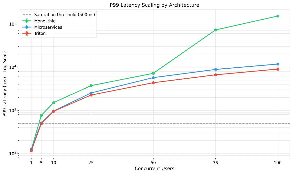
No architecture wins on every axis. The efficiency leader is the tail-latency disaster; the tail-latency leader carries the deployment and memory cost; the throughput leader costs twice the code. That three-way tension is the finding — not a ranking.

Evidence · Figure 1

Three architectures agree, until they don't

Log-scale plot of P99 latency against concurrent users for three serving architectures. From 1 to 25 users all three lines rise together from roughly 120 ms to between 2,500 and 4,000 ms, crossing a 500 ms saturation threshold at around 5 users. At 50 users the monolithic line separates from the other two and climbs steeply to about 152,000 milliseconds — 152 seconds — at 100 users, while microservices reaches about 11,800 ms and Triton about 9,000 ms. The finding is the divergence: the three are indistinguishable until 50 users, then monolithic fails by more than an order of magnitude. — Up to roughly 50 concurrent users the three architectures are indistinguishable — a benchmark that stopped there would report a tie. Past that point monolithic serving diverges by more than an order of magnitude, ending at a P99 of 152 s while the two distributed styles stay near 9–12 s. The log axis is what makes that visible: on a linear axis the entire useful range would be flattened against the baseline by the one architecture that failed.fig. 1 — p99 latency scaling by architecture · log y-axis · 2957×1761

Evidence · Decision framework

Multi-dimensional architecture comparison

Read this as a trade-off surface, not a scoreboard. Every column wins somewhere and loses somewhere, and the right choice depends entirely on which row is binding for your deployment — picking a column means accepting whatever it costs you three rows down. Nothing here dominates.

tab. 1 — decision framework · 7 dimensions × 3 architectures
Dimension	Monolithic	Microservices	Triton
Latency (P99 at 100 users)	152 s (spike risk)	11.8 s	9.0 s (stable)
Throughput	11.6 RPS	14.3 RPS	11.5 RPS
Efficiency (RPS/vCPU)	5.8 (best)	3.5	2.9
Memory footprint	163 MB	1.5 GB	4.0 GB
Code volume	1.0× (baseline)	2.0×	1.4×
Deployment time	50 s (1.0×)	64 s (1.3×)	410 s (8.3×)
Tail latency stability	Unpredictable	Moderate	Stable

Eleven pre-registered hypotheses

7Supported
3Not supported
1Partial

The hypotheses were registered before the runs. Three of them were wrong — most notably, dynamic batching showed no measurable benefit in this workload regime, against the expectation that it would help. A pre-registration that confirms everything is not a pre-registration, so the failed three are reported at the same weight as the seven.

Experiment scale

Matrix

63 tests across the full experiment matrix, all three architectures

Pipeline

A matched two-stage CV pipeline — object detection, then image classification

Config

Every experimental parameter in one experiment.yaml

Abstract

Selecting a machine learning serving architecture is a central design decision in CPU-constrained deployments, which are common in cost-sensitive and edge environments. While the choice directly affects latency compliance, resource cost and operational maintainability, controlled comparative evidence for choosing among architectures remains limited.

This work presents a reproducible evaluation framework for ML serving architectures and instantiates it in a controlled comparison of three deployment styles: monolithic services, microservices, and NVIDIA Triton Inference Server. The framework separates workload specification, controlled-variable alignment, multidimensional measurement and decision synthesis, so that each part can be reused across studies rather than rebuilt per experiment.

Using a matched multi-model detection-classification pipeline, we observe a clear three-way trade-off. Monolithic serving is the most resource-efficient — 5.8 requests/vCPU against 2.9–3.5 for the distributed alternatives — but it exhibits severe tail-latency degradation under high load, reaching a P99 of 152 s at 100 concurrent users. Triton provides the most stable tails (P99/P50 = 1.07) but incurs the highest memory overhead and an 8.28× longer deployment time. Microservices deliver the highest throughput, 23% above the alternatives, through asynchronous fan-out, at approximately 2× code volume.

In this CPU-constrained setting, Triton tensor transport raises network I/O by up to 59× versus the monolithic baseline, while dynamic batching shows no measurable benefit in this workload regime. Of eleven pre-registered hypotheses, seven were supported, three were not, and one was partially supported. The released artifact links workload definitions, measurement scripts and analysis outputs to support transparent replication.

研究摘要

在 CPU 受限的部署環境裡，要選哪一種 ML serving 架構，其實沒有太多可以直接參考的對照證據。這份研究做的是一套可重現的評估框架，並且用它實際比較三種部署方式：單體式、微服務，以及 NVIDIA Triton。

結果是一個三方權衡，沒有哪一種架構在每個面向都贏。單體式的資源效率最好（5.8 requests/vCPU，分散式只有 2.9 到 3.5），但高負載時尾端延遲會崩掉——100 個並行使用者下 P99 是 152 秒。Triton 的尾端最穩定（P99/P50 = 1.07），代價是記憶體用量最高、部署時間長了 8.28 倍。微服務的吞吐量最高（高出 23%），但程式碼量大約是兩倍。

另外一個意外的發現是：在這個規模下，Triton 的 tensor transport 讓網路 I/O 變成單體式基準的 59 倍，而 dynamic batching 完全沒有可測量到的效益。十一個事前登記的假設裡有三個不成立，這一個就是其中之一。那個 59 倍的數字，後來就變成第二個研究的起點。

What was built

The repository is the artifact

The framework is not a description of an experiment — it is the running system that produced every number on this page, and it re-runs from a single configuration file.

Runtime

Python 3.11+, managed with uv; lint by ruff and mypy, format by black

Tests

88% coverage against a stated 80% threshold, enforced in CI

Deployment

Containerized deploys, gRPC between microservices, infrastructure-as-code

Load

Locust load generation driven by a custom runner.py

Observability

Prometheus, Grafana and an OpenTelemetry collector; MinIO for model storage

Reproducibility

All experimental parameters in one experiment.yaml — a single source of truth across all 63 tests, plus static code metrics that produced the code-volume row above

All of it is in the repository linked at the top of this page.

The 59× network result was a question, not a conclusion

If transport dominates compute, does batching at the transport layer fix it? That question became the second project.